CFMRI GE MR750 Imaging Protocol Documentation
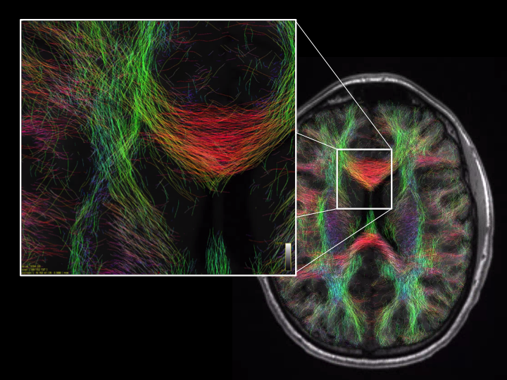
Diffusion Tensor Imaging User Guide
Due to recent updates in GE MRI scanner availability at CFMRI and software version changes, this section is under review and will be updated to reflect current recommendations. Please contact cfmri@ucsd.edu if you have questions or comments on any of the following info.
Introduction
CFMRI supports the following 3 non-multiband DTI protocols
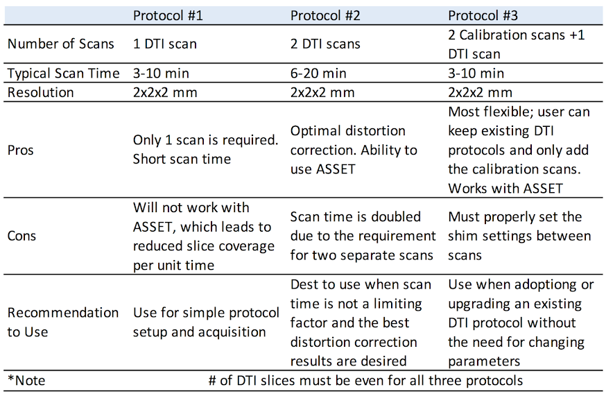
Protocol #1
Description
Protocol #1 consists of DTI acquisition: “DTI‐TOPUP”
By default Protocol 1 acquires two T2 (or b=0) images at the beginning of the scan
The first T2 image uses reversed phase encoding direction, whereas the second T2 image and the subsequent diffusion weighted images use forward phase encoding direction
Due to the requirement of opposite phase encoding directions, the number of T2 images must be 2 or greater.
Location of the Protocol
Adult ‐> Templates ‐> DTI_TOPUP The protocol is available on both 3T West and 3T East scanners.
Parameters
User should adjust b value and number of directions to fit study needs
Other parameters to customize include: FOV, slice thickness, number of slices (must be even), TR, and matrix size.
Advanced Options
The following CVs are set under the advanced tab and can be customized as needed:
CV1: pepolar = 2 or 3 (do not set to 0 or 1)
The pepolar parameter controls the phase encoding direction, i.e. pepolar = 2 corresponds to forward phase encoding, whereas pepolar = 3 corresponds to reverse phase encoding
In a typically MRI setup, forward phase encoding causes compression of the frontal lobe and stretching of the occipital lobe; whereas reverse phase encoding causes stretching of the frontal lobe and compression of the occipital lobe
Since stretching is easier to correct than compression, one could choose this parameter accordingly for the specific areas of brain being studied
CV2: rhmethod = 1
prevent interpolation to 256 in the reconstructed images)
CV4: ssgr fat suppression = 1
reverses spin echo refusing gradient polarity to better suppress fat signal
Shim Settings and Scan Instructions
Shim is set to Auto. After saving Rx, press Scan to start.
Protocol #2
Description
Protocol 2 consists of two DTI acquisitions: “ DTI-fwd” & “DTI-rvs”
The DTI‐fwd scan acquires data in forward phase encoding direction, whereas the DTI‐rvs scan acquires data with reversed phase encoding direction
All parameters must match between the two scans except the phase encoding direction
This protocol is also available with ASSET option ON.
Location of the Protocol
Adult ‐> Templates ‐> DTI_TOPUP The protocol is available on both 3T West and 3T East scanners.
Parameters
User should set the number of T2 images, the number of diffusion directions and b value as desired
The same parameters must be applied to both scans
Other parameters to customize include: * FOV * Slice thickness * Number of slices (must be even) * TR * Matrix size
The same parameters must be applied to both scans
Advanced Options
The following CVs are set under the advanced tab and can be customized as needed:
CV2: rhmethod = 1 * Prevent interpolation to 256 in the reconstructed images
CV4: ssgr fat suppression = 1 * Reverses spin echo refusing gradient polarity to reduce remaining fat signal
Shim Settings and Scan Instructions
The order of the two scans can be swapped. However, the first scan can have shim set to Auto and the second scan must have the shim set to OFF.
For each scan, save Rx and press Scan.
Protocol #3
Description
Protocol 3 consists of three DTI acquisitions: “ DTI”, “DTI_cal_fwd” & “DTI_cal_rvs”
The first two scans of this protocol are calibration scans with forward and reversed phase encoding directions respectively
They are used to estimate the field map, which is then applied to the DTI scan to correct distortions
The subsequent DTI can be any DTI scan (i.e, either GE standard DTI or the DTI supplied with this protocol)
The only requirement is that the Rx info must match among all three scans, e.g. FOV, slice thickness, number of slices and matrix size
This protocol is also available with ASSET option ON
Location of the Protocol
Adult ‐> Templates ‐> DTI_TOPUP The protocol is available on both 3T West and 3T East scanners.
Parameters
For the two calibration scans, user may customize: * FOV * Slice thickness * Number of slices (must be even) * TR * Matrix size Please keep in mind that Rx information must match the DTI scan.
For the DTI, user should set: * Number of T2 images * The number of diffusion directions * b value.
Other parameters to customize include: * FOV * Slice thickness * Number of slices (must be even) * TR * Matrix size
Remember that the Rx info of the DTI scan must match the Rx info of the calibration scans
Advanced Options
User should not change any advanced options in the calibrations scans.
For the DTI scan, if you are using the GE standard DTI, no change should be made in the advanced tab
If you are using the DTI supplied with this protocol, the following CVs under the advanced tab can be customized as needed:
CV1: pepolar = 0 or 1 (do not set to 2 or 3) * The pepolar parameter controls the phase encoding direction, i.e. pepolar = 0 corresponds to forward phase encoding, whereas pepolar = 1 corresponds to reverse phase encoding * In a typically MRI setup, forward phase encoding causes compression of the frontal lobe and stretching of the occipital lobe; whereas reverse phase encoding causes stretching of the frontal lobe and compression of the occipital lobe * Since stretching is easier to correct than compression, one could choose this parameter accordingly for the specific areas of brain being studied
CV2: rhmethod = 1 * To prevent interpolation in the reconstructed images
CV4: ssgr fat suppression = 1 * Reverse spin echo refusing gradient polarity to reduce remaining fat signal
Shim Settings and Scan Instructions
The order of the two scans can be swapped. However, the first scan can have shim set to Auto and the second scan must have the shim set to OFF.
For each scan, save Rx and press Scan.
DTI TOPUP Distortion Correction
Required Software
We provide a C‐Shell script “processtopup” for processing the data acquired with the above protocols.Processtopup first prepares the GE dicom data and converts it into NIFTI format and then calls the TOPUP tool from FSL to unwarp the distortion. More information on the FSL TOPUP tool is available at the FSLwiki website (http://fsl.fmrib.ox.ac.uk/fsl/fslwiki/topup).
Processtopup (http://fmri.ucsd.edu/download/processtopup )
FSL version 5.0 or above (http://fsl.fmrib.ox.ac.uk/fsl/fslwiki/)
Environment Variable FSLOUTPUTTYPE must be set to NIFTI_GZ
Environment Variable FSLDIR must be set and point to the FSL installation folder
The acquired DTI data must have an even number of slices (requirement of the FSL TOPUP tool) * If the number of slices is odd, processtopup will remove the last slice from the data
Usage
processtopup ‐dsnum <num of DTI dir> ‐d1 <data dir> [‐d2 <data dir> ‐d3 <data dir> <options>] ‐o <outstem>”
Required Inputs
‐dsnum <number of DTI data directories, 1, 2 or 3>
if ‐dsnum 1 ‐d1 <DTI data dir>
if ‐dsnum 2 ‐d1 <DTI_fwd data dir> ‐d2 <DTI_rvs data dir>
if ‐dsnum 3 ‐d1 <Cal1_dir> ‐d2 <Cal2_dir>” ‐d3 <DTI data dir>
Note
The ‐d1 and ‐d3 inputs must have the same phase encoding direction;
‐o <unwarpped filename stem>”
Optional Inputs
‐tmpdir : specify tmp dir name ‐nocleanup : disables removal of temporary files
Output
<outstem> ‐ unwarpped volume filename stem
Examples
Protocol 1: >>processtopup ‐dsnum 1 ‐d1 dti_dir ‐o myoutput
Protocol 2: >> processtopup ‐dsnum 2 ‐d1 dti_fwd ‐d2 dti_rvs ‐o myoutput
Protocol 3: >> processtopup ‐dsnum 3 ‐d1 cal_fwd ‐d2 cal_rvs ‐d3 dti_fwd ‐o myoutput
For questions about this manual, please contact Aaron Jacobson (ajacobson@ucsd.edu)
NOTE: Due to recent updates in GE MRI scanner availability at CFMRI and software version changes, this section is under review and will be updated to reflect current recommendations.
Arterial Spin Labeling User Guide
Due to recent updates in GE MRI scanner availability at CFMRI and software version changes, this section is under review and will be updated to reflect current recommendations. Please contact cfmri@ucsd.edu if you have questions or comments on any of the following info.
Background
At CFMRI, we strive to provide the state-of-the-art arterial spin labeling (ASL) protocols for a quick and robust measure of whole brain cerebral blood flow (CBF).
As of May 1, 2015, we have updated our existing ASL protocols to ensure that the scan parameters are in compliance with those recommended by the ISMRM Perfusion Study Group1.
In addition to the standard acquisition parameters, we now provide two additional subsets of parameters optimized for pediatric and geriatric populations.
The scans for each protocol are also more streamlined, making them easier to execute and less prone to operator error.
For questions about the ASL protocols, please contact Conan Chen (coc004@ucsd.edu).
ASL FAQs
What is ASL?
What types of ASL protocols are available at CFMRI?
What is new as of the May 1, 2015 update?
Where do I find the updated CFMRI ASL protocols?
How do I transfer data acquired from the scanner?
How do I process data once the data are acquired?
Between FAIR and PCASL, which one should I use?
Between 2D PCASL and 3D PCASL, which one should I use?
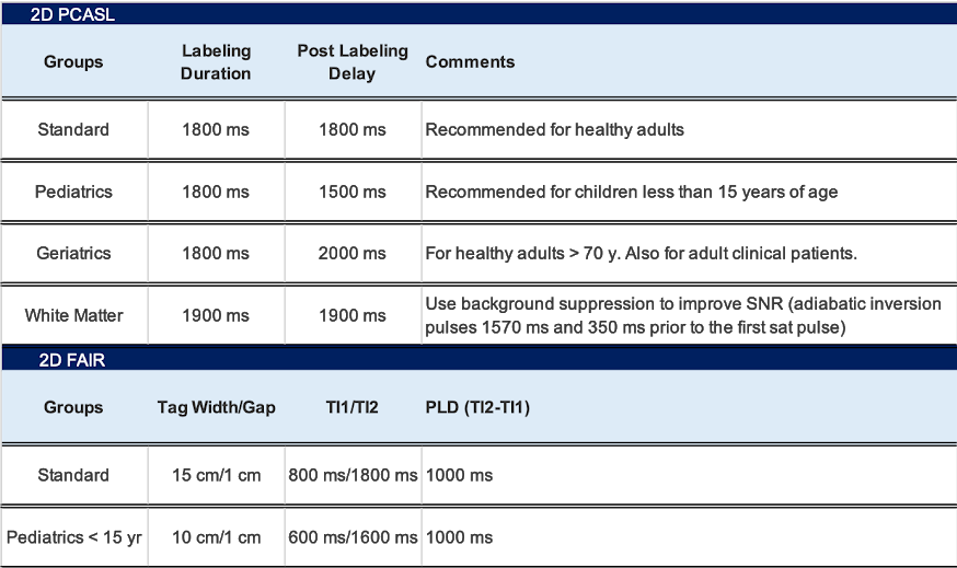
What are the standard scan and labeling parameters for each protocol?
Is there an ASL protocol I can use for functional studies?
What other ASL techniques are out there?
What is ASL?
Healthy brain function is critically dependent on well-regulated CBF for the delivery of oxygen and glucose. Regional alterations in CBF have been observed in a wide range of health conditions, including acute and chronic cerebrovascular disease (e.g. stroke, transient ischemic attacks), Alzheimer’s disease, mild cognitive impairment, epilepsy, HIV-related cognitive impairment, multiple sclerosis, depression, schizophrenia, post-traumatic stress disorder, traumatic brain injury, obsessive-compulsive disorder, and vascular dementia. Over the past decade, ASL has emerged as a robust and non-invasive method for acquiring regional CBF maps. Because of its non-invasive nature and ease of use, a growing number of research and clinical sites are now using ASL.
What types of ASL are available at CFMRI?
We provide both FAIR2 and Pseudocontinuous ASL1 (PCASL) protocols.
What is new in ASL at CFMRI?
In addition to the existing CFMRI 2D PCASL, we now support GE 3DASL.
The CSF scan is now part of the ASL scan and thus is no longer needed as a separate acquisition (no need to remember to run manual prescan!).
Introduced a 10-minute 2D PCASL protocol with background suppression optimized for measurements of whole brain white matter CBF3.
Introduced a single-click multi-TI transit delay mapping protocol (PCASL) that provides a whole brain T1 map, transit delay map, and a quantified CBF map in 15 minutes4.
After the ASL/CSF scan, a MATLAB script is automatically invoked and the quantified CBF map is displayed on screen to provide immediate feedback on data quality.
In order to account for variance in transit delays among different study groups, acquisition parameters have been optimized for each (see below).
Where do I find the updated CFMRI ASL protocols?
The latest ASL protocols are available both on the 3TW and 3TE scanners under
Adult–>Templates–> * C_ASL_2DFAIR * C_ASL_2DPCASL * C_ASL_3DPCASL
Note
Individual scans under each protocol can be selected and imported into your own protocol.
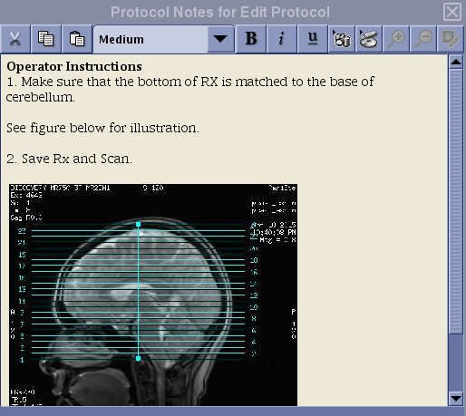
For each of the protocols selected, users will find a note associated with the ASL scan (see red box in the figure above) that describes how to prescribe the imaging volume
How to see the Protocol Note:
Set up a patient and select an ASL protocol
Select a desired ASL series in the Work Flow Manger List Window by a single mouse click on the series and then click on Set Up.
The note will appear directly on the scan prescription page at the right bottom corner (see Figure below).
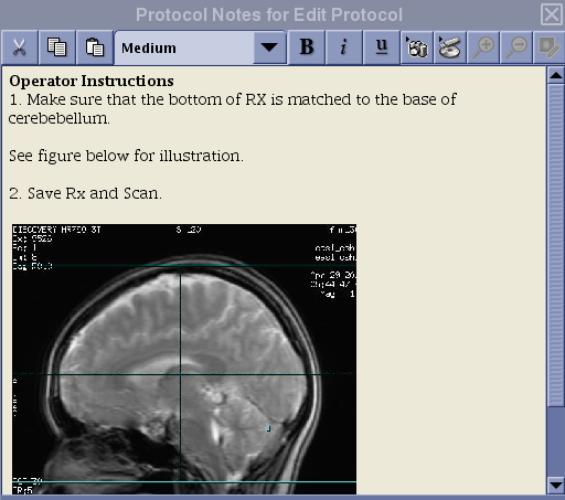
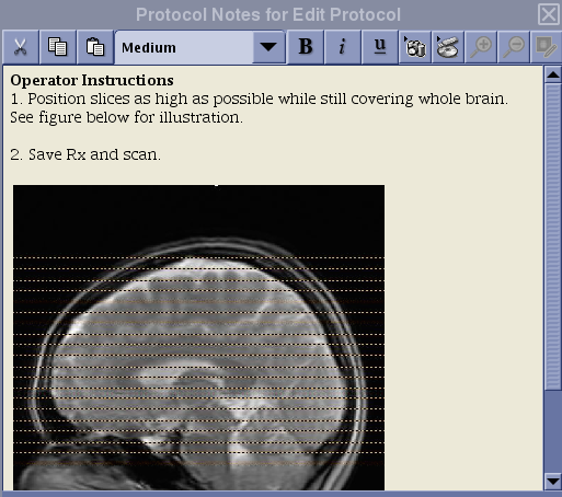
Below are the screenshots of the note for each protocol.
2D PCASL Protocol Coverage
3D PCASL Protocol Coverage
FAIR Protocol Coverage
Note
The prescription instruction for the FAIR protocol is different from that of the PCASL protocols!
N.B. If you erase the default graphic prescription preloaded with the protocol, make sure to position the first line of the graphic tool from the bottom and add slices toward the top. For ASL, the slices must be acquired from bottom to top for proper quantification. Do not place the first line of the graphic tool at the top and extend slices toward the bottom of the head!
How do I transfer data acquired from the scanner?
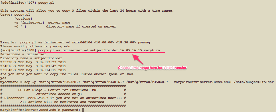
For all protocols other than GE 3DPCASL, the scanner outputs images in GE Pfile format (e.g. P34816.7).
To locate and transfer Pfiles to another server, see example below:
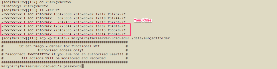
If you have several Pfiles to transfer, it may be easier to use the pcopy.pl script that allows you to transfer files in batch.
Example of how the script can be used is shown below.
For 3DPCASL, T1 structural, and field map scans, data are stored in DICOM format.
Refer to this link for instructions on how to move DICOM files from the scanner to another server.
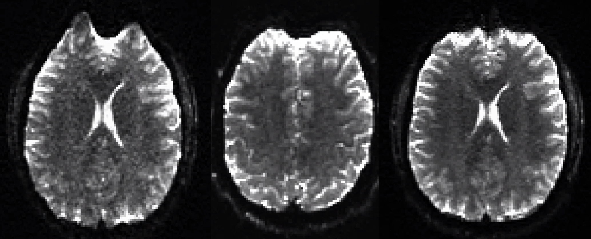
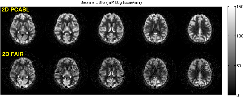
Between FAIR and PCASL, which one should I use?
PCASL is a newer technique that provides several advantages over FAIR. Unless you have an ongoing ASL study using the FAIR protocol, we currently recommend all new users to choose the PCASL protocols.
FAIR and 2D PCASL CBF maps acquired from the same subject are shown below.
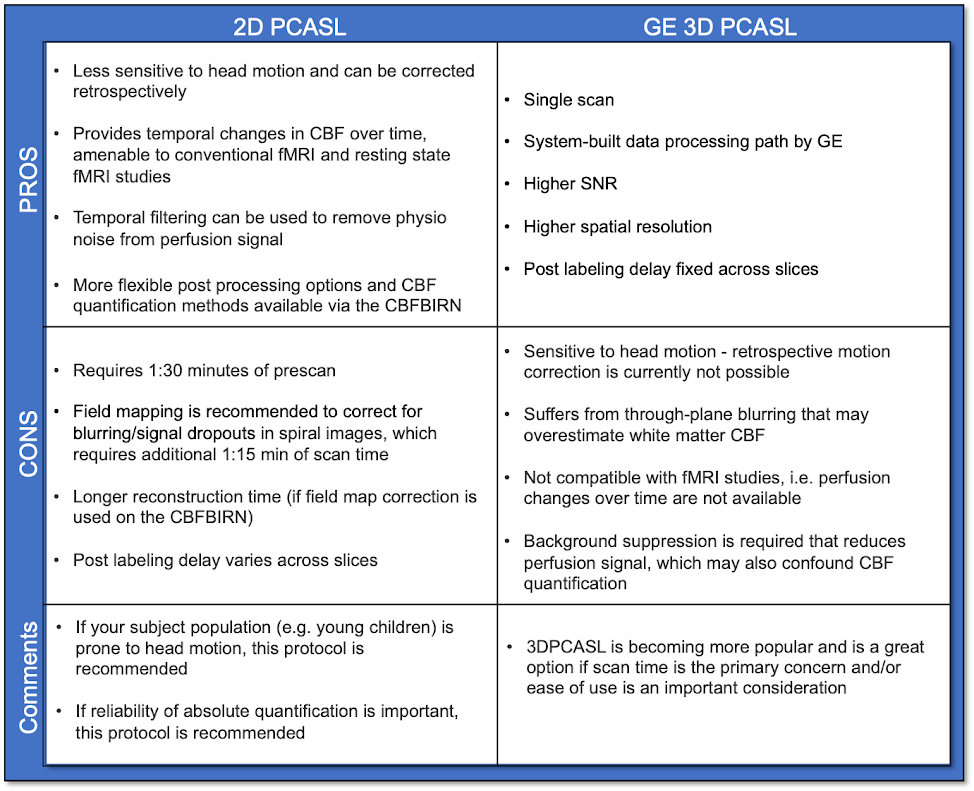
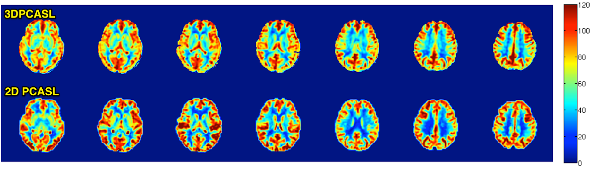
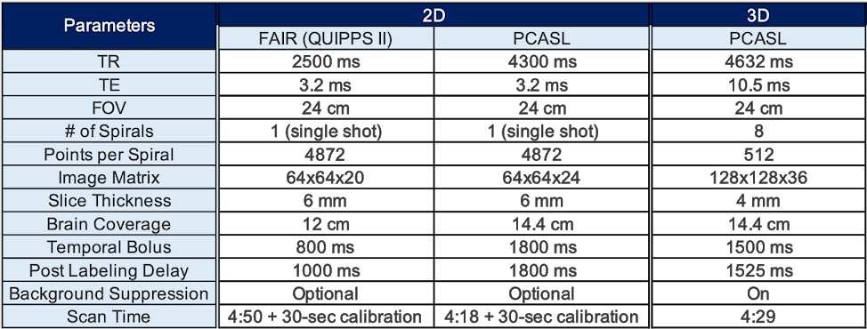
Between 2D PCASL and 3DPCASL, which one should I use?
Use the table below to assess the pros and cons of each protocol.
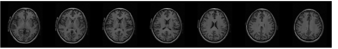
3DPCASL and 2D PCASL CBF maps acquired from the same subject are shown below.
Also shown are corresponding anatomical images.
What are the standard scan and labeling parameters for each protocol?
Dual echo OptPCASL provides both BOLD and ASL time series simultaneously6,7,8.
If OptPCASL is used for a series of functional scans, the same scan can be used to acquire whole brain CBF in the same time it takes to use regular 2D PCASL but with improved labeling efficiency.
Please contact Conan Chen if you are interested in using the OptPCASL protocol for fMRI studies.
What other ASL techniques are out there?
We are actively involved in the development and testing of advanced ASL techniques. Some examples include velocity selective ASL9 and vascular territory imaging10.
If you are interested in using these techniques for your study, please contact Conan Chen (coc004@ucsd.edu).
References
Alsop et al. Recommended implementation of arterial spin-labeled perfusion MRI for clinical applications: A consensus of the ISMRM perfusion study group and the European consortium for ASL in dementia. MRM 73:102-116, 2014.
Wong et al. Quantifying CBF With Pulsed ASL: Technical and Pulse Sequence Factors. JMRI 22:727-731, 2005.
Jia et al. White Matter Perfusion Measurement using Velocity-Selective Arterial Spin Labeling – A Comparison with Pulsed ASL and Pseudo-Continuous ASL. Abstract #2702. ISMRM 2014.
Jia et al. Comparison of Transit Delay Sensitivity between Pseudo-Continuous ASL, Pulsed ASL and Velocity-Selective ASL. Abstract #2705. ISMRM 2014. ISMRM 2014.
Shin et al. The Cerebral Blood Flow Biomedical Informatics Research Network (CBFBIRN) database and analysis pipeline for arterial spin labeing MRI data. Front Neuroinform 7:21, 2012.
Shin et al. Pseudocontinuous Arterial Spin Labeling with Optimized Tagging Efficiency. MRM 68:1135-44, 2012.
Restom et al. Calibrated fMRI in the medial temporal lobe during a memory-encoding task. NeuroImage 40:1495, 2008.
Restom et al. Cerebral Blood Flow and BOLD Responses to a Memory Encoding Task: A Comparison Between Healthy Young and Elderly Adults. NeuroImage 37:430, 2007.
Wong et al. Velocity-selective arterial spin labeling. MRM 55:1334-1341, 2006.
Wong et al. Vessel-Encoded Arterial Spin-Labeling Using Pseudocontinuous Tagging. MRM 58:1086-1091, 2007.